VectorBT Pro - Aligning MTF time series Data with Resampling

Software Requirements : vectorbtpro, python3

Resampling of the market data is needed for strategies that involve multiple time frames, often referred to as “top down analysis” or “Multi Time Frame (MTF) analysis”. There are two types of resampling, called upsampling and downsampling.

Before thinking of upsampling and downsampling time-series data, let's use the analogy of an UltraHD (4K)  television to better understand these terms intuitively. When you feed a 1080p video source to a 4K TV it will Upsample the pixels, giving you a high resolution image. Essentially, you will get a high granularity (finer, hi-res image) from a low granularity (coarse, low-res image). The opposite ( downsampling ) happens when you play a 4K video file on an old 📺 HD TV.

In the context of time series data,

In multi-time frame strategy analysis, we have to deal with the problem of integrating time series data (eg: close price) from multiple time frames.

To make our data-analytics and back-testing simulation process easier, we usually like to have a single time-series dataframe ( mtf_df ) which contains all the values from whatever time-frames we require (eg: 5m, 15min, 1h. 4h, 1D, 1W etc.) . This MTF dataframe will have a base-line frequency which will typically be the highest frequency (i.e highest granularity or the lowest timeframe time-series data, eg: 5m ) with which you want to do your signal generation for the strategy. The process of creating this MTF dataframe with resampled data is called Alignment.

In alignment, we basically merge the MTF time-series  resampled data into a single dataframe using ffill() and shift() operations. This is very easily done using vbt.resampler() objects and using those resampler objects as an argument in vbt.resample_opening() function for open price and vbt.resample_closing() when dealing with close, high, low prices and indicators.

Loading and Resampling Data

Loading the data using vbt.HDF functionality of the 1-minute granularity

## Import Required Libaries
import vectorbtpro as vbt
import pandas as pd

## Load m1 data
m1_data = vbt.HDFData.fetch('../data/GU_OHLCV_3Y.h5')
m1_data.wrapper.index #pandas doaesn't recognise the frequency because of missing timestamps

Output:

DatetimeIndex(['2019-08-27 00:00:00+00:00', '2019-08-27 00:01:00+00:00',
               '2019-08-27 00:02:00+00:00', '2019-08-27 00:03:00+00:00',
               '2019-08-27 00:04:00+00:00', '2019-08-27 00:05:00+00:00',
               '2019-08-27 00:06:00+00:00', '2019-08-27 00:07:00+00:00',
               '2019-08-27 00:08:00+00:00', '2019-08-27 00:09:00+00:00',
               ...
               '2022-08-26 16:50:00+00:00', '2022-08-26 16:51:00+00:00',
               '2022-08-26 16:52:00+00:00', '2022-08-26 16:53:00+00:00',
               '2022-08-26 16:54:00+00:00', '2022-08-26 16:55:00+00:00',
               '2022-08-26 16:56:00+00:00', '2022-08-26 16:57:00+00:00',
               '2022-08-26 16:58:00+00:00', '2022-08-26 16:59:00+00:00'],
              dtype='datetime64[ns, UTC]', name='time', length=1122468, freq=None)

Resampling (Downsampling) the Data from 1 Minute Timeframe / Granularity to other Timeframes/Granularities.

• Converting 1 Minute (M1) to 15 Minute (M15)
• Converting 1 Minute (M1) to 1 Hour (H1)
• Converting 1 Minute (M1) to 4 Hours (H4)

This resampling uses the vbt.resample() method for the downsampling operations, after which we see the frequency is identified correctly as 15T (15 mins)

m15_data = m1_data.resample('15T')
h1_data = m1_data.resample("1h")
h4_data = m1_data.resample('4h')
print(m15_data.wrapper.index)

Output:

DatetimeIndex(['2019-08-27 00:00:00+00:00', '2019-08-27 00:15:00+00:00',
               '2019-08-27 00:30:00+00:00', '2019-08-27 00:45:00+00:00',
               '2019-08-27 01:00:00+00:00', '2019-08-27 01:15:00+00:00',
               '2019-08-27 01:30:00+00:00', '2019-08-27 01:45:00+00:00',
               '2019-08-27 02:00:00+00:00', '2019-08-27 02:15:00+00:00',
               ...
               '2022-08-26 14:30:00+00:00', '2022-08-26 14:45:00+00:00',
               '2022-08-26 15:00:00+00:00', '2022-08-26 15:15:00+00:00',
               '2022-08-26 15:30:00+00:00', '2022-08-26 15:45:00+00:00',
               '2022-08-26 16:00:00+00:00', '2022-08-26 16:15:00+00:00',
               '2022-08-26 16:30:00+00:00', '2022-08-26 16:45:00+00:00'],
              dtype='datetime64[ns, UTC]', name='time', length=105188, freq='15T')

As seen in the code below the respective (OHLC) can be obtained using the .get() method.

# Obtain all the closing  prices using the .get() method
m15_close = m15_data.get()['Close']

## h1 data
h1_open  = h1_data.get()['Open']
h1_close = h1_data.get()['Close']
h1_high  = h1_data.get()['High']
h1_low   = h1_data.get()['Low']

## h4 data
h4_open  = h4_data.get()['Open']
h4_close = h4_data.get()['Close']
h4_high  = h4_data.get()['High']
h4_low   = h4_data.get()['Low']

OR, you can can also simply follow the pandas convention like resampled_data.column_name to retrieve the column data

# Obtain all the closing  prices using the .get() method
m15_close = m15_data.close

## h1 data
h1_open  = h1_data.open
h1_close = h1_data.close
h1_high  = h1_data.high
h1_low   = h1_data.low

## h4 data
h4_open  = h4_data.open
h4_close = h4_data.close
h4_high  = h4_data.high
h4_low   = h4_data.low

The OHLC for both the H4 4-Hourly Candle Data as well as the closing price for the 15m Candle Data was obtained.

Multi-Time Frame Indicator Creation

VectorBT has a built-in method called vbt.talib() which calls the required indicator from talib library and runs it on the specified time-series data (Eg: Close Price or another indicator). We will now create the following indicators (manually) on the M15, H1 and H4 timeframes using the :

• RSI of 21 period
• BBANDS Bolllinger Bands
• BBANDS_RSI Bollinger Bands on the RSI

rsi_period = 21

## 15m indicators
m15_rsi = vbt.talib("RSI", timeperiod = rsi_period).run(m15_close, skipna=True).real.ffill()
m15_bbands = vbt.talib("BBANDS").run(m15_close, skipna=True)
m15_bbands_rsi = vbt.talib("BBANDS").run(m15_rsi, skipna=True)

## h4 indicators
h1_rsi = vbt.talib("RSI", timeperiod = rsi_period).run(h1_close, skipna=True).real.ffill()
h1_bbands = vbt.talib("BBANDS").run(h1_close, skipna=True)
h1_bbands_rsi = vbt.talib("BBANDS").run(h1_rsi, skipna=True)

## h4 indicators
h4_rsi = vbt.talib("RSI", timeperiod = rsi_period).run(h4_close, skipna=True).real.ffill()
h4_bbands = vbt.talib("BBANDS").run(h4_close, skipna=True)
h4_bbands_rsi = vbt.talib("BBANDS").run(h4_rsi, skipna=True)

When talib() creates the RSI indicator time-series, it is known to create it with NaNs (null-values), so it is a good idea to run ffill(), forward filling operation to fill the missing values. On this note, it is also a good idea in general, to investigate the talib results and compare it with the original time-series data (Close Price) for abnormal number of NaN values and then decide on ffill() operation

We will now initialize the empty dict called data and fill it with key - value pairs of the 15m time-series data.

## Initialize  dictionary
data = {}

col_values = [
    m15_close, m15_rsi, m15_bbands.upperband, m15_bbands.middleband, m15_bbands.lowerband, 
    m15_bbands_rsi.upperband, m15_bbands_rsi.middleband, m15_bbands_rsi.lowerband
    ]

col_keys = [
    "m15_close", "m15_rsi", "m15_bband_price_upper",  "m15_bband_price_middle", "m15_bband_price_lower", 
    "m15_bband_rsi_upper",  "m15_bband_rsi_middle", "m15_bband_rsi_lower"
         ]

# Assign key, value pairs for method of time series data to store in data dict
for key, time_series in zip(col_keys, col_values):
    data[key] = time_series.ffill()

Alternative (One-Liner) Method of Indicator Creation

VectorBT also offers a more convenient one-liner method of creating this multi-time frame indicators

rsi_period = 21

rsi = vbt.talib("RSI", timeperiod=rsi_period).run(
    m15_data.get("Close"), 
    timeframe=["15T", "1H" , "4H"], 
    skipna=True, 
    broadcast_kwargs=dict(wrapper_kwargs=dict(freq="15T"))
).real

bbands_price = vbt.talib("BBANDS").run(
    m15_data.get("Close"), 
    timeframe=["15T", "1H", "4H"], 
    skipna=True,
    broadcast_kwargs=dict(wrapper_kwargs=dict(freq="15T"))
)

bbands_rsi = vbt.talib("BBANDS").run(
    rsi,
    timeframe=vbt.Default(["15T", "1H" ,"4H"]),
    skipna=True,
    per_column=True,
    broadcast_kwargs=dict(wrapper_kwargs=dict(freq="15T"))
)

Note : The method of indicator creation shown above using talib('IndicatorName').run with broadcast_kwargs argument automatically does the ffill() operation. This one liner method doesn't resample to 15T only because of broadcast_kwargs argument, in fact, using broadcast_kwargs we just provide vbt with the true frequency of your data in case this frequency cannot be inferred from data. Without specifying it the method will still work (we will just get a warning if frequency cannot be inferred)
So here we we specify the broadcast_kwargs argument, because m15_data.get("Close") contains gaps and pandas cannot infer its frequency as 15T, this approach works only because of the timeframe argument and because indicators always return outputs of the same index as their inputs, such that we're forced to resample it back to the original frequency. If pandas can infer the frequency of the input series, we don't need to specify broadcast_kwargs argument at all.

## Initialize  dictionary
data = {}

## Assign key, value pairs for method 2 of Automated One-liner MTF indicator creation method
col_values = [
    [m15_close.ffill(), rsi['15T'], bbands_price['15T'].upperband, bbands_price['15T'].middleband, bbands_price['15T'].lowerband, bbands_rsi['15T'].upperband, bbands_rsi['15T'].middleband, bbands_rsi['15T'].lowerband],
    [rsi['1H'], bbands_price['1H'].upperband, bbands_price['1H'].middleband, bbands_price['1H'].lowerband, bbands_rsi['1H'].upperband, bbands_rsi['1H'].middleband, bbands_rsi['1H'].lowerband],
    [rsi['4H'], bbands_price['4H'].upperband, bbands_price['4H'].middleband, bbands_price['4H'].lowerband, bbands_rsi['4H'].upperband, bbands_rsi['4H'].middleband, bbands_rsi['4H'].lowerband]
    ]

col_keys = [
    ["m15_close", "m15_rsi", "m15_bband_price_upper",  "m15_bband_price_middle", "m15_bband_price_lower",  "m15_bband_rsi_upper",  "m15_bband_rsi_middle", "m15_bband_rsi_lower"], 
    ["h1_rsi", "h1_bband_price_upper",  "h1_bband_price_middle",  "h1_bband_price_lower",  "h1_bband_rsi_upper",  "h1_bband_rsi_middle", "h1_bband_rsi_lower"],
    ["h4_rsi", "h4_bband_price_upper",  "h4_bband_price_middle",  "h4_bband_price_lower",  "h4_bband_rsi_upper",  "h4_bband_rsi_middle", "h4_bband_rsi_lower" ],
         ]

## Assign key, value pairs for method 2 of Automated One-liner MTF indicator creation method
for lst_series, lst_keys in zip(col_values, col_keys):
    for key, time_series in zip(lst_keys, lst_series):
        data[key] = time_series

Alignment & Up-sampling

Let's now see what is resampler in VectorBT. Resampler is an instance of the Resampler class, which simply stores a source index and frequency, and a target index and frequency. The vbt.resampler() method can just work with the source index and target index and can automatically infer the source and target frequency. In contrast to Pandas, vectorbt can also accept an arbitrary target index for resampling

Resampler(
    source_index,
    target_index,
    source_freq=None,
    target_freq=None,
    silence_warnings=None
)

where the arguments, are

source_index : is index_like, Index being resampled.
target_index : is index_like ,Index resulted from resampling.
source_freq : frequency_like or bool, Frequency or date offset of the source index. Set to False to force-set the frequency to None.
target_freq : frequency_like or bool, Frequency or date offset of the target index. Set to False to force-set the frequency to None.
silence_warnings : bool, Whether to silence all warnings.

We will now create a custom function called create_resamplers() using this vbt.Resampler() function to create a resampler object to convert H4 time-series

def create_resamplers(result_dict_keys_list : list, source_indices : list,  
                      source_frequencies :list, target_index : pd.Series, target_freq : str):
    """
    Creates a dictionary of vbtpro resampler objects.

    Parameters
    ==========
    result_dict_keys_list : list, list of strings, which are keys of the output dictionary
    source_indices        : list, list of pd.time series objects of the higher timeframes
    source_frequencies    : list(str), which are short form representation of time series order. Eg:["1D", "4h"]
    target_index          : pd.Series, target time series for the resampler objects
    target_freq           : str, target time frequency for the resampler objects

    Returns
    ===========
    resamplers_dict       : dict, vbt pro resampler objects
    """
    
    
    resamplers = []
    for si, sf in zip(source_indices, source_frequencies):
        resamplers.append(vbt.Resampler(source_index = si,  target_index = target_index,
                                        source_freq = sf, target_freq = target_freq))
    return dict(zip(result_dict_keys_list, resamplers))

Using this function we can create a dictionary of vbt.Resampler objecters stored by appropriately named keys.

## Create Resampler Objects for upsampling
src_indices = [h1_close.index, h4_close.index]
src_frequencies = ["1H","4H"] 
resampler_dict_keys = ["h1_m15","h4_m15"]

list_resamplers = create_resamplers(resampler_dict_keys, src_indices, src_frequencies, m15_close.index, "15T")

print(list_resamplers)

Output:

{'h1_m15': <vectorbtpro.base.resampling.base.Resampler at 0x16c83de70>,
 'h4_m15': <vectorbtpro.base.resampling.base.Resampler at 0x16c5478e0>}

The output shows that two vbt.Resampler class objects have been created in memory.

The resample_closing() and resample_opening() operations don't require any ffill() operations and they automatically align the source time-series data to the target frequency, which in our case is 15T (15 mins)

## Add H1 OLH data - No need to do ffill() on resample_closing as it already does that by default
data["h1_open"] = h4_open.vbt.resample_opening(list_resamplers['h1_m15'])

## Add H4 OLH data - No need to do ffill() on resample_closing as it already does that by default
data["h4_open"] = h4_open.vbt.resample_opening(list_resamplers['h4_m15'])

We use resample_opening only if information in the array happens exactly at the beginning of the bar (such as open price), and resample_closing if information happens after that (such as high, low, and close price). You can see the effect of this resample_opening operation with the print() statements below:

print(h4_open.info()) ## Before resampling pandas series

<class 'pandas.core.series.Series'>
DatetimeIndex: 6575 entries, 2019-08-27 00:00:00+00:00 to 2022-08-26 16:00:00+00:00
Freq: 4H
Series name: Open
Non-Null Count  Dtype  
--------------  -----  
4841 non-null   float64
dtypes: float64(1)
memory usage: 102.7 KB
None

print(data["h4_open"].info()) ## After resampling pandas series

<class 'pandas.core.series.Series'>
DatetimeIndex: 105188 entries, 2019-08-27 00:00:00+00:00 to 2022-08-26 16:45:00+00:00
Freq: 15T
Series name: Open
Non-Null Count   Dtype  
--------------   -----  
105188 non-null  float64
dtypes: float64(1)
memory usage: 1.6 MB
None

## Use along with  Manual indicator creation method for MTF
series_to_resample = [
    [h1_high, h1_low, h1_close, h1_rsi, 
    h1_bbands.upperband, h1_bbands.middleband, h1_bbands.lowerband,
    h1_bbands_rsi.upperband, h1_bbands_rsi.middleband, h1_bbands_rsi.lowerband], 
    [h4_high, h4_low, h4_close, h4_rsi,
    h4_bbands.upperband, h4_bbands.middleband, h4_bbands.lowerband, 
    h4_bbands_rsi.upperband, h4_bbands_rsi.middleband, h4_bbands_rsi.lowerband]
    ]

data_keys = [
    ["h1_high", "h1_low", "h1_close", "h1_rsi", 
    "h1_bband_price_upper", "h1_bband_price_middle","h1_bband_price_lower", 
     "h1_bband_rsi_upper",  "h1_bband_rsi_middle", "h1_bband_rsi_lower"],
    ["h4_high", "h4_low", "h4_close", "h4_rsi", 
    "h4_bband_price_upper", "h4_bband_price_middle", "h4_bband_price_lower", 
     "h4_bband_rsi_upper",  "h4_bband_rsi_middle", "h4_bband_rsi_lower"]
     ]

## Create resampled time series data aligned to base line frequency (15min)

for lst_series, lst_keys, resampler in zip(series_to_resample, data_keys, resampler_dict_keys):
    for key, time_series in zip(lst_keys, lst_series):
        resampled_time_series = time_series.vbt.resample_closing(list_resamplers[resampler])
        data[key] = resampled_time_series

Alignment and Resampling when using one-liner method of indicator creation

In this method, we have already dealt with resampling and aligning the indicators, so all we have to do is just resample the open and closing prices of the respective timeframes required.

## Resample prices to match base_line frequency (`15T`)

series_to_resample = [
    [h1_open, h1_high, h1_low, h1_close],
    [h4_open, h4_high, h4_low, h4_close]
    ]

data_keys = [
    ["h1_open", "h1_high", "h1_low", "h1_close"],
    ["h4_open", "h4_high", "h4_low" ,"h4_close"]
    ]

## Create resampled time series data aligned to base line frequency (15min)

for lst_series, lst_keys, resampler in zip(series_to_resample, data_keys, resampler_dict_keys):
    for key, time_series in zip(lst_keys, lst_series):
        if key.lower().endswith('open'):
            print(f'Resampling {key} differently using vbt.resample_opening using "{resampler}" resampler')
            resampled_time_series = time_series.vbt.resample_opening(list_resamplers[resampler])
        else:
            resampled_time_series = time_series.vbt.resample_closing(list_resamplers[resampler])
        data[key] = resampled_time_series

Creating The Master DataFrame

Now that we have resampled the various time series to the different timeframes, created and run our indicators, we can finally create the composite mtf_df dataframe from this data which is properly aligned to the baseline frequency (in our case 15T) that will allow us to properly create the Buy/Long and Sell/Short conditions for whichever MTF (Multi Time Frame) Strategy that we indend to backtest.

cols_order = ['m15_close', 'm15_rsi', 'm15_bband_price_upper','m15_bband_price_middle', 'm15_bband_price_lower',
              'm15_bband_rsi_upper','m15_bband_rsi_middle', 'm15_bband_rsi_lower',
              'h1_open', 'h1_high', 'h1_low', 'h1_close', 'h1_rsi',
              'h1_bband_price_upper', 'h1_bband_price_middle', 'h1_bband_price_lower', 
              'h1_bband_rsi_upper', 'h1_bband_rsi_middle', 'h1_bband_rsi_lower',              
              'h4_open', 'h4_high', 'h4_low', 'h4_close', 'h4_rsi',
              'h4_bband_price_upper', 'h4_bband_price_middle', 'h4_bband_price_lower', 
              'h4_bband_rsi_upper', 'h4_bband_rsi_middle', 'h4_bband_rsi_lower'
              ]

## construct a multi-timeframe dataframe
mtf_df = pd.DataFrame(data)[cols_order]
display(mtf_df)            

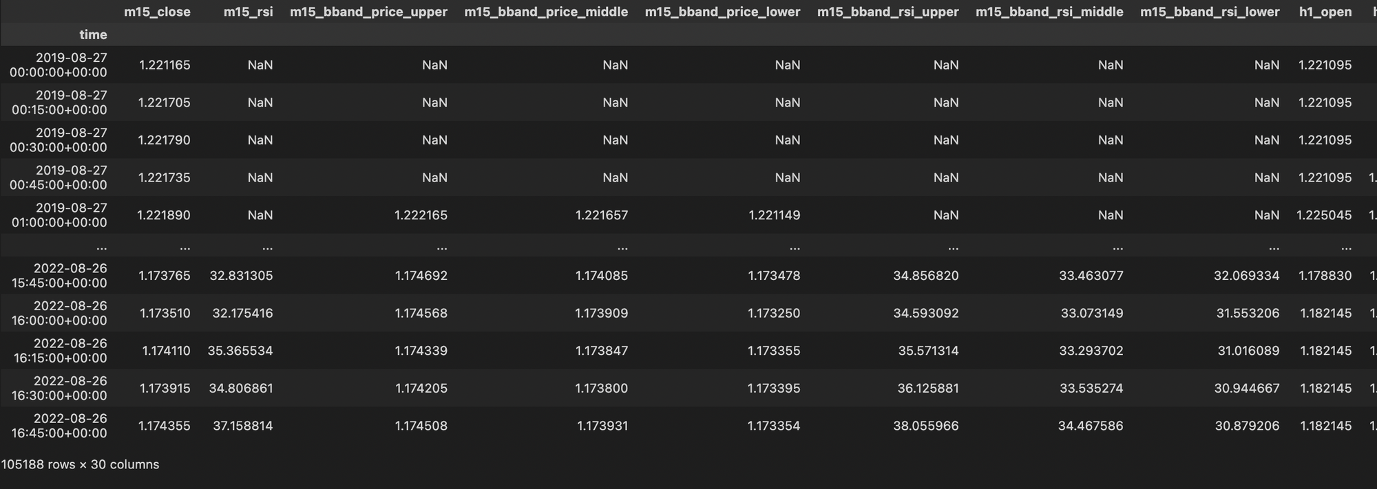
The mtf_df multi-time frame master dataframe will have the following columns each of which will help us define the logic of the strategy.

1. m15_close : 15 Minute Closing Price
2. m15_rsi : RSI values on the m15closing price of period 21
3. m15_bband_price_upper: The upper bollinger band on m15 closing price
4. m15_bband_price_middle: The middle bollinger band on m15 closing price
5. m15_bband_price_lower : The lower bollinger band on m15 closing price
6. m15_bband_rsi_upper : The Upper Bollinger Band on the M15 RSI Values
7. m15_bband_rsi_middle : The Middle Bollinger Band on the M15 RSI Values
8. m15_bband_rsi_lower: The Lower Bollinger band on the M15 RSI Values
9. h1_open: The opening price of the H1 candle
10. h1_high: The High Price of the H1 Candle
11. h1_low: The Low Price of the H1 Candle
12. h1_close: The Closing Price of the H1 Candle
13. h1_rsi : RSI Values on the H1 closing price of period 21
14. h1_bband_price_upper: The Upper Bollinger Band On H1 Closing Price
15. h1_bband_price_middle: The Middle Bollinger Band On H1 Closing Price
16. h1_bband_price_lower:The Lower Bollinger Band On H1 Closing Price
17. h1_bband_rsi_upper: The Upper Bollinger Band on the H1 RSI Value
18. h1_bband_rsi_middle: The Middle Bollinger Band on the H1 RSI Value
19. h1_bband_rsi_lower: The Lower Bollinger Band on the H1 RSI Value
20. h4_open: The opening price of the H4 candle
21. h4_high: The High Price of the H4 Candle
22. h4_low: The Low Price of the H4 Candle
23. h4_close: The Closing Price of the H4 Candle
24. h4_rsi : RSI Values on the H4 closing price of period 21
25. h4_bband_price_upper: The Upper Bollinger Band On H4 Closing Price
26. h4_bband_price_middle: The Middle Bollinger Band On H4 Closing Price
27. h4_bband_price_lower:The Lower Bollinger Band On H4 Closing Price
28. h4_bband_rsi_upper: The Upper Bollinger Band on the H4 RSI Value
29. h4_bband_rsi_middle: The Middle Bollinger Band on the H4 RSI Value
30. h4_bband_rsi_lower: The Lower Bollinger Band on the H4 RSI Value

print(mtf_df.info())

<class 'pandas.core.frame.DataFrame'>
DatetimeIndex: 105188 entries, 2019-08-27 00:00:00+00:00 to 2022-08-26 16:45:00+00:00
Freq: 15T
Data columns (total 33 columns):
 #   Column                  Non-Null Count   Dtype  
---  ------                  --------------   -----  
 0   m15_close               105188 non-null  float64
 1   m15_rsi                 105167 non-null  float64
 2   m15_bband_price_upper   105184 non-null  float64
 3   m15_bband_price_middle  105184 non-null  float64
 4   m15_bband_price_lower   105184 non-null  float64
 5   m15_bband_rsi_upper     105163 non-null  float64
 6   m15_bband_rsi_middle    105163 non-null  float64
 7   m15_bband_rsi_lower     105163 non-null  float64
 8   h1_open                 105188 non-null  float64
 9   h1_high                 105185 non-null  float64
 10  h1_low                  105185 non-null  float64
 11  h1_close                105185 non-null  float64
 12  h1_rsi                  105101 non-null  float64
 13  h1_bband_price_upper    105169 non-null  float64
 14  h1_bband_price_middle   105169 non-null  float64
 15  h1_bband_price_lower    105169 non-null  float64
 16  h1_bband_rsi_upper      105085 non-null  float64
 17  h1_bband_rsi_middle     105085 non-null  float64
 18  h1_bband_rsi_lower      105085 non-null  float64
 19  h4_open                 105188 non-null  float64
 20  h4_high                 105173 non-null  float64
 21  h4_low                  105173 non-null  float64
 22  h4_close                105173 non-null  float64
 23  h4_rsi                  104837 non-null  float64
 24  h4_bband_price_upper    105109 non-null  float64
 25  h4_bband_price_middle   105109 non-null  float64
 26  h4_bband_price_lower    105109 non-null  float64
 27  h4_bband_rsi_upper      104773 non-null  float64
 28  h4_bband_rsi_middle     104773 non-null  float64
...
 32  signal                  105188 non-null  int64  
dtypes: bool(2), float64(30), int64(1)
memory usage: 29.9 MB

Summary

In general, the resampling and alignment steps for creating a multi-time frame (MTF) dataframe can be summarized in the below diagram.

1. We start with the highest granularity of OHLCV data possible (1m) and then downsample the data to higher timeframes (5m, 15m, 1h, 4h etc.)
2. We then create the indicators on the multiple time frames required but at this juncture we don't forward fill the price data. After the indicator is created we can ffill() the resulting series if we are going with the manual method of indicator creation.
3. In order to create the composite, merged MTF dataframe we employ resample_opening() on the open price or resample_closing() on every other time series, with the appropriate vbt.Resampler() objects, so that all the time-series are aligned to the base-line frequency time series.