
VectorBT Pro - MultiAsset Portfolio Simulation

In this tutorial, we will talk about verious topics pertaining to Multi Asset Portfolio Simulation, beginning with
- Converting various forex (FX) pairs to the account currency, if the quote currency of the currency pair is not the same as the account currency.
- Running different types of backtesting simulations like
grouped,unifiedanddiscreteusingvbt.Portfolio.from_signals(), and - Finally, exporting data to
.picklefiles for plotting and visualizing in an interactive plotly dashboard.
Before proceeding further, you would want to read this short helper tutorial about multi-asset data acquisition which explains how we created the below
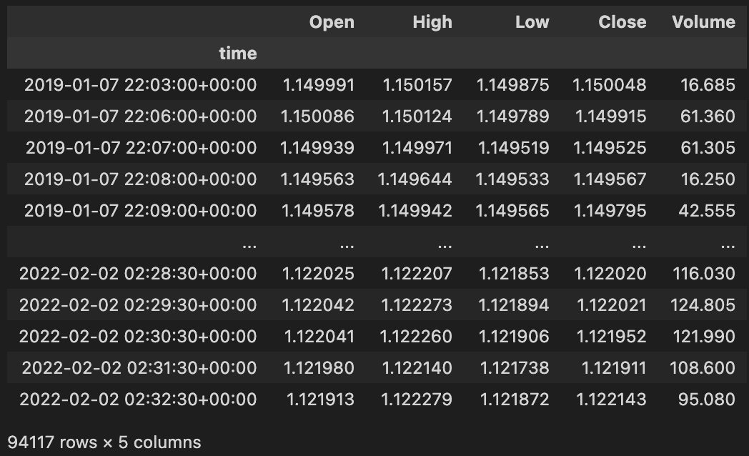
MultiAsset_OHLCV_3Y_m1.h5file, which we load intohdf_data
Here, we will run the Double Bollinger Band Strategy from our earlier tutorial on multiple assets. But before we do that, we have to bring the quote value of all our forex currency pairs to the account currency (USD).
## Import Libraries
import numpy as np
import pandas as pd
import vectorbtpro as vbt

## Forex Data
hdf_data = vbt.HDFData.fetch('/Users/dilip.rajkumar/Documents/vbtpro_tuts_private/data/MultiAsset_OHLCV_3Y_m1.h5')
symbols = hdf_data.symbols
print('Multi-Asset DataFrame Symbols:',symbols)
Output
Multi-Asset DataFrame Symbols: ['AUDUSD', 'EURGBP', 'EURUSD', 'GBPAUD', 'GBPJPY', 'GBPUSD', 'USDCAD', 'USDJPY']
Convert FX pairs where quote_currency != account currency ( US$ )
We will be converting OHLC price columns for the following currency pairs to the account currency (USD), as in these pairs either the quote currency or both the base currency & quote currency are not the same as the account currency which in our requirement is USD.
price_cols = ["Open", "High", "Low", "Close"]
symbols_to_convert = ["USDJPY", "USDCAD", "GBPJPY", "EURGBP", "GBPAUD"]
For this currency conversion of price data, we will use this convert_to_account_currency function, which handles the following scenarios, where the quote currency is not the same as account currency:
1.) Base currency == Account currency :
In this case, we simply inverse the price of the instrument. For eg: in the case of USDJPY the quote currency is JPY, but the base currency is the same as the account currency (USD). So in order to get the price of USDJPY in USD all we have to do is compute 1 / USDJPY.
2.) Both (Base Currency & Quote Currency ) != Account Currency :
This scenario occurs when we basically don't see the account currency characters in the source forex currency pair symbol (Eg: GBPJPY) and in order to convert this kind of currency pair to the account currency we require a bridge currency pair. Now depending on how the bridge pair symbol is presented in the market data provided by the exchange, we would be either dividing or multiplying the source currency pair by the bridge pair. For eg:
a.) In the case of converting GBPJPY to USD, we would be dividing GBPJPY / USDJPY
b.) In the case of converting GBPAUD to USD, the exchange typically provides the bridge currency pair data required as AUDUSD and not USDAUD and so in this case, we would be multiplying GBPAUD * AUDUSD.
def convert_to_account_currency(price_data : pd.Series, account_currency : str = "USD",
                                bridge_pair_price_data: pd.Series = None) -> pd.Series:
    """
    Convert prices of different FX pairs to account currency.

    Parameters
    ==========
    price_data      :   pd.Series, Price data from (OHLC) columns of the pair to be converted
    account_currency:   str, default = 'USD'
    bridge_pair_price_data: pd.Series, price data to be used when neither,
                            the base or quote currency is = account currency

    Returns
    =======
    new_instrument_price : pd.Series, converted price data

    """
    symbol = price_data.name
    base_currency  = symbol[0:3].upper()
    quote_currency = symbol[3:6].upper() ## a.k.a Counter_currency

    if base_currency == account_currency: ## case 1  - Eg: USDJPY
        print(f"BaseCurrency: {base_currency} is same as AccountCurrency: {account_currency} for Symbol:- {symbol}."+ \
              "Performing price inversion")
        new_instrument_price = (1/price_data)

    elif (quote_currency != account_currency) and (base_currency != account_currency): ## Case 2 - Eg: GBPJPY
        bridge_pair_symbol =  account_currency + quote_currency  ## Bridge Pair symbol is : USDJPY
        print(f"Applying currency conversion for {symbol} with {bridge_pair_symbol} price data")
        if (bridge_pair_price_data is None):
            raise Exception(f"Price data for {bridge_pair_symbol} is missing. Please provide the same")
        elif (bridge_pair_symbol != bridge_pair_price_data.name.upper()):
            message = f"Mismatched data. Price data for {bridge_pair_symbol} is expected, but" + \
                      f"{bridge_pair_price_data.name.upper()} price data is provided"
            print(message) ## Eg: When AUDUSD is required, but instead USDAUD is provided
            new_instrument_price = price_data * bridge_pair_price_data
            # raise Exception(message)
        else:
            new_instrument_price = price_data/ bridge_pair_price_data ## Divide GBPJPY / USDJPY

    else:
        print(f"No currency conversion needed for {symbol} as QuoteCurreny: {quote_currency} == Account Currency")
        new_instrument_price = price_data
    return new_instrument_price
We copy the data from the original hdf_data file and store them in a dictionary of dataframes. For symbols whose price columns are to be converted we create an empty pd.DataFrame which we will be filling with the converted price values
new_data = {}
for symbol, df in hdf_data.data.items():
    if symbol in symbols_to_convert: ## symbols whose price columns needs to be converted to account currency
        new_data[symbol] = pd.DataFrame(columns=['Open','High','Low','Close','Volume'])
    else: ## for other symbols store the data as it is
        new_data[symbol] = df
Here we call our convert_to_account_currency() function to convert the price data to account cuurency. For pairs like USDJPY and USDCAD a simple price inversion (Eg: 1 / USDJPY ) alone is sufficient, so for these cases we will be setting bridge_pair == None.
bridge_pairs = [None, None, "USDJPY", "GBPUSD", "AUDUSD"]

for ticker_source, ticker_bridge  in zip(symbols_to_convert, bridge_pairs):
    new_data[ticker_source]["Volume"] = hdf_data.get("Volume")[ticker_source]
    for col in price_cols:
        print("Source Symbol:", ticker_source, "|| Bridge Pair:", ticker_bridge, "|| Column:", col)
        new_data[ticker_source][col] = convert_to_account_currency(
                            price_data =  hdf_data.get(col)[ticker_source],
                            bridge_pair_price_data = None  if ticker_bridge is None else hdf_data.get(col)[ticker_bridge]
                            )
Ensuring Correct data for High and Low columns
Once we have the converted OHLC price columns for a particular symbol (ticker_source), we recalculate the High and Low by getting the max and min of each row in the OHLC columns respectively using df.max(axis=1) and df.min(axis=1)
## Converts this `new_data` (dict of dataframes) into a vbt.Data object
m1_data = vbt.Data.from_data(new_data)

for ticker_source in symbols:
    m1_data.data[ticker_source]['High'] = m1_data.data[ticker_source][price_cols].max(axis=1)
    m1_data.data[ticker_source]['Low'] = m1_data.data[ticker_source][price_cols].min(axis=1)
What need is there for above step?
Lets assume for a symbol X if low is 10 and high is 20, then when we do a simple price inversion ( 1/X ) new high would become 1/10 = 0.1 and new low would become 1/20 = 0.05 which will result in complications and thus arises the need for the above step
## Sanity check to see if empty pd.DataFrame got filled now
m1_data.data['EURGBP'].dropna()
Double Bollinger Band Strategy over Multi-Asset portfolio
The following steps are very similar we already saw in the Alignment and Resampling and Strategy Development tutorials, except now they are applied over multiple symbols (assets) in a portfolio. So I will just put the code here and won't be explaining anything here in detail, when in doubt refer back to the above two tutorials.
m15_data = m1_data.resample('15T')  # Convert 1 minute to 15 mins
h1_data = m1_data.resample("1h")    # Convert 1 minute to 1 hour
h4_data = m1_data.resample('4h')    # Convert 1 minute to 4 hour

# Obtain all the required prices using the .get() method
m15_close = m15_data.get('Close')

## h1 data
h1_open  = h1_data.get('Open')
h1_close = h1_data.get('Close')
h1_high  = h1_data.get('High')
h1_low   = h1_data.get('Low')

## h4 data
h4_open  = h4_data.get('Open')
h4_close = h4_data.get('Close')
h4_high  = h4_data.get('High')
h4_low   = h4_data.get('Low')

### Create (manually) the indicators for Multi-Time Frames
rsi_period = 21

## 15m indicators
m15_rsi = vbt.talib("RSI", timeperiod = rsi_period).run(m15_close, skipna=True).real.ffill()
m15_bbands = vbt.talib("BBANDS").run(m15_close, skipna=True)
m15_bbands_rsi = vbt.talib("BBANDS").run(m15_rsi, skipna=True)

## h1 indicators
h1_rsi = vbt.talib("RSI", timeperiod = rsi_period).run(h1_close, skipna=True).real.ffill()
h1_bbands = vbt.talib("BBANDS").run(h1_close, skipna=True)
h1_bbands_rsi = vbt.talib("BBANDS").run(h1_rsi, skipna=True)

## h4 indicators
h4_rsi = vbt.talib("RSI", timeperiod = rsi_period).run(h4_close, skipna=True).real.ffill()
h4_bbands = vbt.talib("BBANDS").run(h4_close, skipna=True)
h4_bbands_rsi = vbt.talib("BBANDS").run(h4_rsi, skipna=True)
def create_resamplers(result_dict_keys_list : list, source_indices : list,
                      source_frequencies :list, target_index : pd.Series, target_freq : str):
    """
    Creates a dictionary of vbtpro resampler objects.

    Parameters
    ==========
    result_dict_keys_list : list, list of strings, which are keys of the output dictionary
    source_indices        : list, list of pd.time series objects of the higher timeframes
    source_frequencies    : list(str), which are short form representation of time series order. Eg:["1D", "4h"]
    target_index          : pd.Series, target time series for the resampler objects
    target_freq           : str, target time frequency for the resampler objects

    Returns
    ===========
    resamplers_dict       : dict, vbt pro resampler objects
    """


    resamplers = []
    for si, sf in zip(source_indices, source_frequencies):
        resamplers.append(vbt.Resampler(source_index = si,  target_index = target_index,
                                        source_freq = sf, target_freq = target_freq))
    return dict(zip(result_dict_keys_list, resamplers))
## Initialize  dictionary
mtf_data = {}

col_values = [
    m15_close, m15_rsi, m15_bbands.upperband, m15_bbands.middleband, m15_bbands.lowerband,
    m15_bbands_rsi.upperband, m15_bbands_rsi.middleband, m15_bbands_rsi.lowerband
    ]

col_keys = [
    "m15_close", "m15_rsi", "m15_bband_price_upper",  "m15_bband_price_middle", "m15_bband_price_lower",
    "m15_bband_rsi_upper",  "m15_bband_rsi_middle", "m15_bband_rsi_lower"
         ]

# Assign key, value pairs for method of time series data to store in data dict
for key, time_series in zip(col_keys, col_values):
    mtf_data[key] = time_series.ffill()

## Create Resampler Objects for upsampling
src_indices = [h1_close.index, h4_close.index]
src_frequencies = ["1H","4H"]
resampler_dict_keys = ["h1_m15","h4_m15"]

list_resamplers = create_resamplers(resampler_dict_keys, src_indices, src_frequencies, m15_close.index, "15T")

## Use along with  Manual indicator creation method for MTF
series_to_resample = [
    [h1_open, h1_high, h1_low, h1_close, h1_rsi, h1_bbands.upperband, h1_bbands.middleband, h1_bbands.lowerband,
     h1_bbands_rsi.upperband, h1_bbands_rsi.middleband, h1_bbands_rsi.lowerband],
    [h4_high, h4_low, h4_close, h4_rsi, h4_bbands.upperband, h4_bbands.middleband, h4_bbands.lowerband,
    h4_bbands_rsi.upperband, h4_bbands_rsi.middleband, h4_bbands_rsi.lowerband]
    ]


data_keys = [
    ["h1_open","h1_high", "h1_low", "h1_close", "h1_rsi", "h1_bband_price_upper",  "h1_bband_price_middle",  "h1_bband_price_lower",
     "h1_bband_rsi_upper",  "h1_bband_rsi_middle", "h1_bband_rsi_lower"],
    ["h4_open","h4_high", "h4_low", "h4_close", "h4_rsi", "h4_bband_price_upper",  "h4_bband_price_middle",  "h4_bband_price_lower",
     "h4_bband_rsi_upper",  "h4_bband_rsi_middle", "h4_bband_rsi_lower"]
         ]

for lst_series, lst_keys, resampler in zip(series_to_resample, data_keys, resampler_dict_keys):
    for key, time_series in zip(lst_keys, lst_series):
        if key.lower().endswith('open'):
            print(f'Resampling {key} differently using vbt.resample_opening using "{resampler}" resampler')
            resampled_time_series = time_series.vbt.resample_opening(list_resamplers[resampler])
        else:
            resampled_time_series = time_series.vbt.resample_closing(list_resamplers[resampler])
        mtf_data[key] = resampled_time_series

cols_order = ['m15_close', 'm15_rsi', 'm15_bband_price_upper','m15_bband_price_middle', 'm15_bband_price_lower',
              'm15_bband_rsi_upper','m15_bband_rsi_middle', 'm15_bband_rsi_lower',
              'h1_open', 'h1_high', 'h1_low', 'h1_close', 'h1_rsi',
              'h1_bband_price_upper', 'h1_bband_price_middle', 'h1_bband_price_lower',
              'h1_bband_rsi_upper', 'h1_bband_rsi_middle', 'h1_bband_rsi_lower',
              'h4_open', 'h4_high', 'h4_low', 'h4_close', 'h4_rsi',
              'h4_bband_price_upper', 'h4_bband_price_middle', 'h4_bband_price_lower',
              'h4_bband_rsi_upper', 'h4_bband_rsi_middle', 'h4_bband_rsi_lower'
              ]
Double Bollinger Band - Strategy Conditions
required_cols = ['m15_close','m15_rsi','m15_bband_rsi_lower', 'm15_bband_rsi_upper',
                 'h4_low', "h4_rsi", "h4_bband_price_lower", "h4_bband_price_upper" ]

## Higher values greater than 1.0 are like moving up the lower RSI b-band,
## signifying if the lowerband rsi is anywhere around 1% of the lower b-band validate that case as True
bb_upper_fract = 0.99
bb_lower_fract = 1.01

## Long Entry Conditions
# c1_long_entry = (mtf_data['h1_low'] <= mtf_data['h1_bband_price_lower'])
c1_long_entry = (mtf_data['h4_low'] <= mtf_data['h4_bband_price_lower'])
c2_long_entry = (mtf_data['m15_rsi'] <= (bb_lower_fract * mtf_data['m15_bband_rsi_lower']) )


## Long Exit Conditions
# c1_long_exit =  (mtf_data['h1_high'] >= mtf_data['h1_bband_price_upper'])
c1_long_exit = (mtf_data['h4_high'] >= mtf_data['h4_bband_price_upper'])
c2_long_exit = (mtf_data['m15_rsi'] >= (bb_upper_fract * mtf_data['m15_bband_rsi_upper']))

## Strategy conditions check - Using m15 and h4 data
mtf_data['entries'] = c1_long_entry & c2_long_entry
mtf_data['exits']  = c1_long_exit & c2_long_exit

mtf_data['signal'] = 0
mtf_data['signal'] = np.where( mtf_data['entries'], 1, 0)
mtf_data['signal'] = np.where( mtf_data['exits'] , -1, mtf_data['signal'])
After the above np.where, we can use this pd.df.where to return a pandas object
mtf_data['signal'] = mtf_data['entries'].vbt.wrapper.wrap(mtf_data['signal'])
mtf_data['signal'] = mtf_data['exits'].vbt.wrapper.wrap(mtf_data['signal'])
print(mtf_data['signal'])
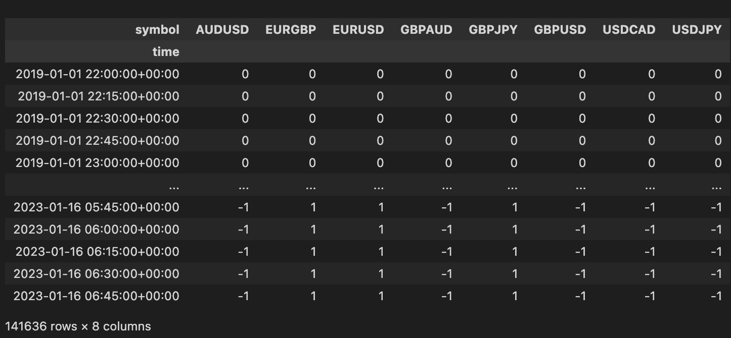
Signal Column for Multiple Forex Pair SymbolsCleaning and Resampling entries and exits
entries = mtf_data['signal'] == 1.0
exits = mtf_data['signal'] == -1.0
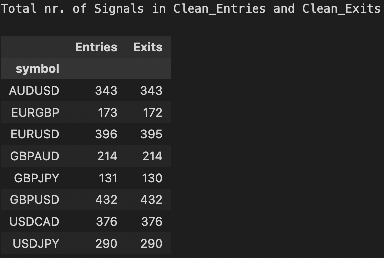
## Clean redundant and duplicate signals
clean_entries, clean_exits = entries.vbt.signals.clean(exits)
print(f"Total nr. of Signals in Clean_Entries and Clean_Exits")
pd.DataFrame(data = {"Entries":clean_entries.vbt.signals.total(),
"Exits": clean_exits.vbt.signals.total()})
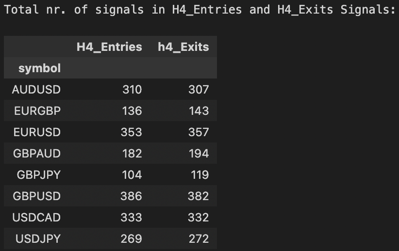
We can resample the entries and exits for plotting purposes on H4 chart, but this always produces some loss in the nr. of signals as the entries / exits in our strategy is based on M15 timeframe. So just be aware of this.
## Resample clean entries to H4 timeframe
clean_h4_entries = clean_entries.vbt.resample_apply("4h", "any", wrap_kwargs=dict(dtype=bool))
clean_h4_exits = clean_exits.vbt.resample_apply("4h", "any", wrap_kwargs=dict(dtype=bool))

print(f"Total nr. of H4_Entry Signals:\n {clean_h4_entries.vbt.signals.total()}\n")
print(f"Total nr. of H4_Exit Signals:\n {clean_h4_exits.vbt.signals.total()}")
Saving Data to .pickle file
For the purposes of plotting, we will be saving various data like:
- price data across various timeframes
- indicator data across various timeframes
- entries & exits
- finally, the
vectorbt.portfolioobjects after running each type of portfolio simulation
## Save Specific Data to pickle file for plotting purposes
price_data = {"h4_data": h4_data, "m15_data" : m15_data}
vbt_indicators = {'m15_rsi': m15_rsi,'m15_price_bbands': m15_bbands, 'm15_rsi_bbands' : m15_bbands_rsi,
                  'h4_rsi': h4_rsi, 'h4_price_bbands':h4_bbands, 'h4_rsi_bbands' : h4_bbands_rsi}

entries_exits_data = {'clean_entries' : clean_entries, 'clean_exits' : clean_exits}

print(type(h4_data), '||' ,type(m15_data))
print(type(h4_bbands), '||', type(h4_bbands_rsi), '||', type(h1_rsi))
print(type(m15_bbands), '||', type(m15_bbands_rsi), '||', type(m15_rsi))

file_path1 = '../vbt_dashboard/data/price_data'
file_path2 = '../vbt_dashboard/data/indicators_data'
file_path3 = '../vbt_dashboard/data/entries_exits_data'


vbt.save(price_data, file_path1)
vbt.save(vbt_indicators, file_path2)
vbt.save(entries_exits_data, file_path3)
Multi-asset Portfolio Backtesting simulation using vbt.Portfolio.from_signals()
In this section, we will see different ways to run this portfolio.from_signals() simulation and save the results as .pickle files to be used in a plotly-dash data visualization dashboard later (in another tutorial).
1.) Asset-wise Discrete Portfolio Simulation
In this section we will see how to run the portfolio simulation for each asset in the portfolio independently. If we start with the default from_signals() function as we had from the previous tutorial, the simulation is run for each symbol independently, which means the account balance is not connected between the various trades executed across symbols
pf_from_signals_v1 = vbt.Portfolio.from_signals(
close = mtf_data['m15_close'],
entries = mtf_data['entries'],
exits = mtf_data['exits'],
direction = "both", ## This setting trades both long and short signals
freq = pd.Timedelta(minutes=15),
init_cash = 100000
)
## Save portfolio simulation as a pickle file
pf_from_signals_v1.save("../vbt_dashboard/data/pf_sim_discrete")
## Load saved portfolio simulation from pickle file
pf = vbt.Portfolio.load('../vbt_dashboard/data/pf_sim_discrete')
## View Trading History of pf.simulation
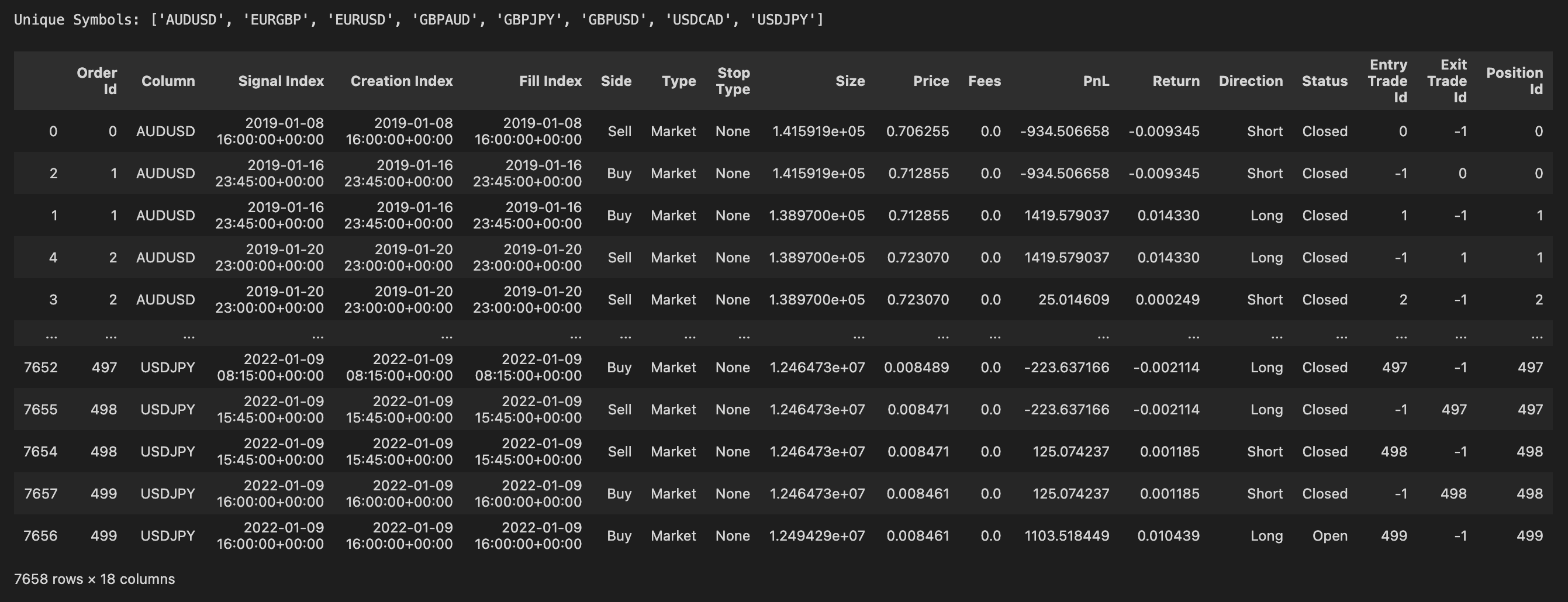
pf_trade_history = pf.trade_history
print("Unique Symbols:", list(pf_trade_history['Column'].unique()) )
pf_trade_history
We can view the portfolio simulation statistics as a dataframe by running the following code snippet
## View Portfolio Stats as a dataframe for pf_from_signals_v1 case
## pd.concat() operation concates the stats information acosss all assets
stats_df = pd.concat([pf.stats()] + [pf[symbol].stats() for symbol in symbols], axis = 1)
## Remove microsend level granularity information in TimeDelta Object
stats_df.loc['Avg Winning Trade Duration'] = [x.floor('s') for x in stats_df.iloc[21]]
stats_df.loc['Avg Losing Trade Duration'] = [x.floor('s') for x in stats_df.iloc[22]]
stats_df = stats_df.reset_index()
stats_df.rename(inplace = True, columns = {'agg_stats':'Agg_Stats', 'index' : 'Metrics' })
stats_df
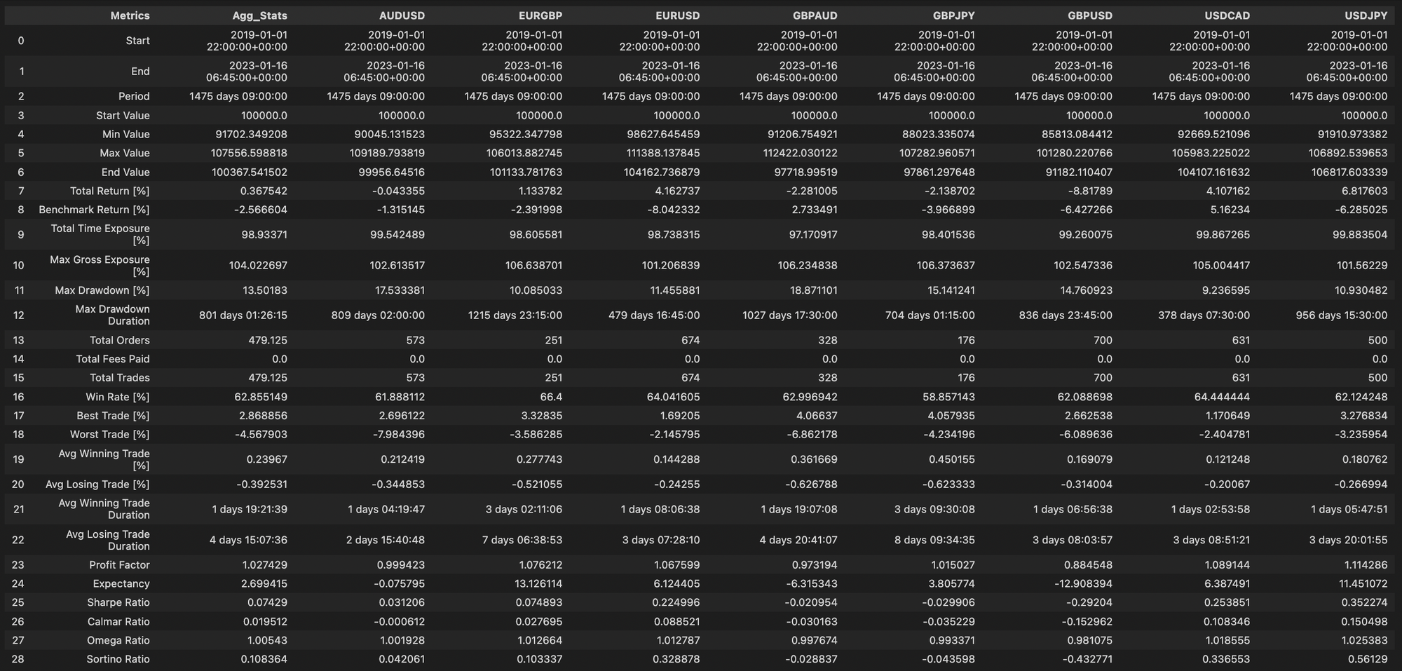
The Agg_Stats column is basically the metrics aggregated across the various symbols which you can validate by running the following code and comparing the output with the above dataframe print out
print("Mean Total Return [%] (across cols):", np.round(np.mean(stats_df.iloc[[7]].values.tolist()[0][1:]), 4) )
print("Mean Total Orders (across cols):", np.round(np.mean(stats_df.iloc[[13]].values.tolist()[0][1:]), 4) )
print("Mean Sortino Ratio (across cols):", np.round(np.mean(stats_df.iloc[[28]].values.tolist()[0][1:]), 4) )
Output:
Mean Total Return [%] (across cols): 0.3675
Mean Total Orders (across cols): 479.125
Mean Sortino Ratio (across cols): 0.1084
Description of a few Parameter settings for pf.from_signals()
We will see a short description of the new parameters of vbt.Portfolio.from_signals() function which we will be using henceforth in the rest of this tutorial.
But I would like to point out that the from_signals() function in VectorBT Pro is very exhaustive in its capabilities and feature set, thus it is beyond the scope of this blog post to cover every parameter of this function along with multitude of settings. So please refer the documentation for this.
a.) size : Specifies the position size in units. For any fixed size, you can set to any number to buy/sell some fixed amount or value. For any target size, you can set to any number to buy/sell an amount relative to the current position or value. If you set this to np.nan or 0 it will get skipped (or close the current position in the case of setting 0 for any target size). Set to np.inf to buy for all cash, or -np.inf to sell for all free cash. A point to remember setting to np.inf may cause the scenario for the portfolio simulation to become heavily weighted to one single instrument. So use a sensible size related.
b.) init_cash : Initial capital per column (or per group with cash sharing). By setting it to auto the initial capital is automatically decided based on the position size you specify in the above size parameter.
c.) cash_sharing : Accepts a boolean (True or False) value to specify whether cash sharing is to be disabled or if enabled then cash is shared across all the assets in the portfolio or cash is shared within the same group.
If group_by is None and cash_sharing is True, group_by becomes True to form a single group with cash sharing. Example:
Consider three columns (3 assets), each having $100 of starting capital. If we built one group of two columns and one group of one column, the init_cash would be np.array([200, 100]) with cash sharing enabled and np.array([100, 100, 100]) without cash sharing.
d.) call_seq : Default sequence of calls per row and group. Controls the sequence in which order_func_nb is executed within each segment. For more details of this function kindly refer the documentation.
e.) group_by : can be boolean, integer, string, or sequence to call multi-level indexing and can accept both level names and level positions. In this tutorial I will be setting group_by = True to treat the entire portfolio simulation in a unified manner for all assets in congruence with cash_sharing = True. When I want to create custom groups with specific symbols in each group then I will be setting group_by = 0 to specify the level position (in multi-index levels) as the first in the hierarchy.
2.) Unified Portfolio Simulation
In this section, we run the portfolio simulation treating the entire portfolio as a singular asset by enabling the following parameters in the pf.from_signals():
cash_sharing = Truegroup_by = Truecall_seq = "auto"size = 100000
pf_from_signals_v2 = vbt.Portfolio.from_signals(
    close = mtf_data['m15_close'],
    entries = mtf_data['entries'],
    exits = mtf_data['exits'],
    direction = "both", ## This setting trades both long and short signals
    freq = pd.Timedelta(minutes=15),
    init_cash = "auto",
    size = 100000,
    group_by = True,
    cash_sharing = True,
    call_seq = "auto"
)

## Save portfolio simulation as a pickle file
pf_from_signals_v2.save("../vbt_dashboard/data/pf_sim_single")

## Load portfolio simulation from pickle file
pf = vbt.Portfolio.load('../vbt_dashboard/data/pf_sim_single')
pf.stats()
Now in this case since the entire portfolio is simulated in a unified manner for all symbols with cash sharing set to True, we get only one pd.Series object for the portfolio simulation stats.
Output
Start                         2019-01-01 22:00:00+00:00
End                           2023-01-16 06:45:00+00:00
Period                               1475 days 09:00:00
Start Value                               781099.026861
Min Value                                  751459.25085
Max Value                                 808290.908182
End Value                                 778580.017067
Total Return [%]                              -0.322496
Benchmark Return [%]                           0.055682
Total Time Exposure [%]                       99.883504
Max Gross Exposure [%]                        99.851773
Max Drawdown [%]                               4.745308
Max Drawdown Duration                 740 days 04:15:00
Total Orders                                       3833
Total Fees Paid                                     0.0
Total Trades                                       3833
Win Rate [%]                                  63.006536
Best Trade [%]                                  4.06637
Worst Trade [%]                               -7.984396
Avg Winning Trade [%]                          0.200416
Avg Losing Trade [%]                          -0.336912
Avg Winning Trade Duration    1 days 12:07:11.327800829
Avg Losing Trade Duration     3 days 22:03:11.201716738
Profit Factor                                  1.007163
Expectancy                                     0.858292
...
Sharpe Ratio                                  -0.015093
Calmar Ratio                                  -0.016834
Omega Ratio                                    0.999318
Sortino Ratio                                 -0.021298
Name: group, dtype: object
3.) Grouped Portfolio Simulation
In this section, we run the portfolio simulation by combining the 8 currency pairs into two groups USDPairs and NonUSDPairs respectively, along with the following parameter settings in the pf.from_signals():
cash_sharing = Truegroup_by = Truecall_seq = "auto"size = 100000
print("Symbols:",list(pf_from_signals_v2.wrapper.columns))
grp_type = ['USDPairs', 'NonUSDPairs', 'USDPairs', 'NonUSDPairs', 'NonUSDPairs', 'USDPairs', 'USDPairs', 'USDPairs']
unique_grp_types = list(set(grp_type))
print("Group Types:", grp_type)
print("Nr. of Unique Groups:", unique_grp_types)
Output:
Symbols: ['AUDUSD', 'EURGBP', 'EURUSD', 'GBPAUD', 'GBPJPY', 'GBPUSD', 'USDCAD', 'USDJPY']
Group Types: ['USDPairs', 'NonUSDPairs', 'USDPairs', 'NonUSDPairs', 'NonUSDPairs', 'USDPairs', 'USDPairs', 'USDPairs']
Nr. of Unique Groups: ['USDPairs', 'NonUSDPairs']
VectorBT expects the group labels to be in a monolithic, sorted array, that is our group must be in a monolithic sorted order like:
[USDPairs, USDPairs, USDPairs, USDPairs, USDPairs, NonUSDPairs, NonUSDPairs, NonUSDPairs] not a random order like:
['USDPairs', 'NonUSDPairs', 'USDPairs', 'NonUSDPairs', 'NonUSDPairs', 'USDPairs', 'USDPairs', 'USDPairs']. So
we create a small method reorder_columns that takes a pandas object and reorders it by sorting columns levels by the level you want to group-by, as a way of preparing the dataframe before it's getting passed to the from_signals() method..
def reorder_columns(df, group_by):
    return df.vbt.stack_index(group_by).sort_index(axis=1, level=0)
Thereafter, we pass group_by=0 (first level) to the pf.from_signals() method before we're running the simulation, since we appended grp_type list of level names, as the top-most level to the columns of each dataframe, thus making it the first in the hierarchy.
pf_from_signals_v3 = vbt.Portfolio.from_signals(
close = reorder_columns(mtf_data["m15_close"], group_by = grp_type),
entries = reorder_columns(mtf_data['entries'], group_by = grp_type),
exits = reorder_columns(mtf_data['exits'], group_by = grp_type),
direction = "both", ## This setting trades both long and short signals
freq = pd.Timedelta(minutes=15),
init_cash = "auto",
size = 100000,
group_by = 0,
cash_sharing=True,
call_seq="auto"
)
## Save portfolio simulation as a pickle file
pf_from_signals_v3.save("../vbt_dashboard/data/pf_sim_grouped")
## Load portfolio simulation from a pickle file
pf = vbt.Portfolio.load('../vbt_dashboard/data/pf_sim_grouped')
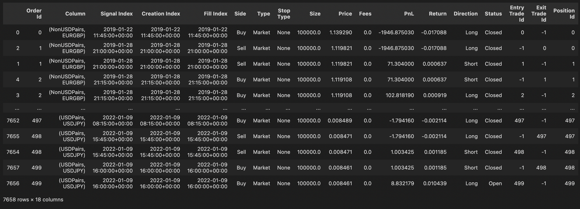
## View Trading History of pf.simulation
pf_trade_history = pf.trade_history
print("Unique Symbols:", list(pf_trade_history['Column'].unique()) )
pf_trade_history
Output:
Unique Symbols: [('NonUSDPairs', 'EURGBP'), ('NonUSDPairs', 'GBPAUD'), ('NonUSDPairs', 'GBPJPY'), ('USDPairs', 'AUDUSD'), ('USDPairs', 'EURUSD'), ('USDPairs', 'GBPUSD'), ('USDPairs', 'USDCAD'), ('USDPairs', 'USDJPY')]
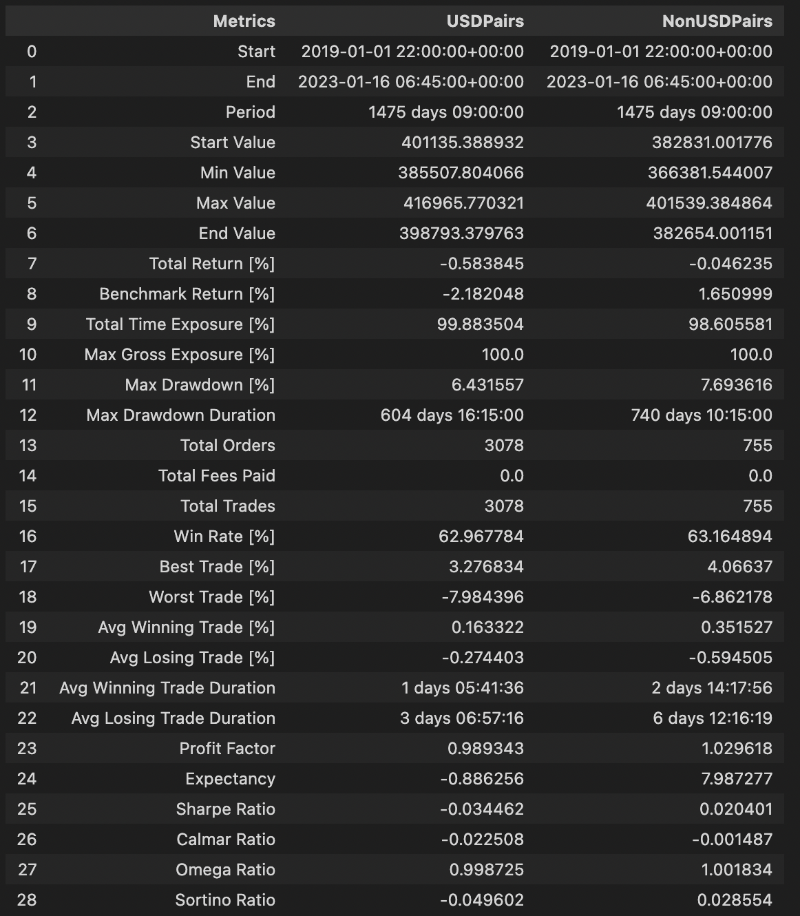
Grouped Portfolio Simulation# For pf_from_signals_v3 case
stats_df = pd.concat([pf[grp].stats() for grp in unique_grp_types], axis = 1)
stats_df.loc['Avg Winning Trade Duration'] = [x.floor('s') for x in stats_df.iloc[21]]
stats_df.loc['Avg Losing Trade Duration'] = [x.floor('s') for x in stats_df.iloc[22]]
stats_df = stats_df.reset_index()
stats_df.rename(inplace = True, columns = {'agg_stats':'Agg_Stats', 'index' : 'Metrics' })
stats_df
This concludes the tutorial for multi-asset portfolio simulation. I hope this is useful in your backtesting studies and workflow. If there are any issues or fixes, please leave a git issue in the link below to the jupyter notebook.